Getting Started with Kaggle Competitions: Melanoma Classification Challenge

This blog gives a gentle introduction for beginners on getting started with Kaggle competitions.

📌 Note: The authors of this blog post jointly participated in the Kaggle competition as a team.

This post assumes that you are acquainted with the basic skills of working with PyTorch. If you are new to PyTorch, we would highly encourage you to go through Deep Leaning With PyTorch: A 60 Minute Blitz by PyTorch. It’s a great place for beginners to get your hands dirty.

Download Data

Here we will be using the preprocessed images by Arnaud Roussel due to storage limitations on Google Colab.

Now let’s download the preprocessed image dataset using the Kaggle API. Remember to add your USERNAME and API_KEY in the code block below.

!pip install kaggle -q
!mkdir /root/.kaggle
!echo '{"username":"YOUR_USERNAME","key":"YOUR_API_KEY"}' > /root/.kaggle/kaggle.json
!chmod 600 /root/.kaggle/kaggle.json
!kaggle datasets download -d arroqc/siic-isic-224x224-images
!mkdir /content/siic-isic-224x224-images
!unzip -q /content/siic-isic-224x224-images.zip -d /content/siic-isic-224x224-images

Download the csv files from the competition page and place this files in the content directory.

!python3 -m pip install --upgrade pip -q
!pip install efficientnet_pytorch pretrainedmodels -q

What is Melanoma?

Malignant Melanoma is a type of skin cancer that develops from pigment-producing cells known as melanocytes.

The skin cells found in the upper layer of the skin are termed as Melanocytes. These produce a pigment Melanin, which is the pigment that is responsible for skin color. Exposure to UV radiation from the sun or tanning beds causes skin damage as it triggers these melanocytes to increase the secretion of Melanin.

Melanoma occurs when there is DNA damage caused by burning or tanning due to UV exposure, triggering mutations in the melanocytes leading to unrestricted cellular growth.

Objective

The objective of this competition is to identify melanoma in images of skin lesions. In particular, we need to use images within the same patient and determine which are likely to represent a melanoma. Using patient-level contextual information may help the development of image analysis tools, which could better support clinical dermatologists.

Melanoma is a deadly disease, but if detected at an early stage, most melanomas can be cured with minor surgery.

This competition is aimed at building a Classification Model that can predict whether the onset of malignant Melanoma from lesion images.

In short, we need to create a classification model that is capable of distinguishing whether the lesion in the image is benign (class 0) or malignant (class 1).

This will be very helpful to detect the early signs so that further medical attention can be made available to the patient.

Now let’s import the necessary packages below.

%matplotlib inline
import os
from tqdm import tqdm
import numpy as np
import pandas as pd
import matplotlib.pyplot as plt
from sklearn.model_selection import StratifiedKFold
from sklearn.metrics import roc_auc_score
import torch
import torch.nn as nn
import torch.nn.functional as F
import torchvision.transforms as transforms
import albumentations
import pretrainedmodels
from efficientnet_pytorch import EfficientNet
from PIL import Image

Now, we select the device on which our network will run. Neural style transfer algorithm runs faster on GPU so check if GPU is available using torch.cuda.is_available().

# device configuration
device = torch.device('cuda' if torch.cuda.is_available() else 'cpu')

About the Dataset

The dataset consists of images and metadata, which are described as follows:

• Images: DICOM, JPEG, TFRecord formats
• Metadata: image_name, patient_id, sex, age_approx, anatom_site_general_challenge, diagnosis, benign_malignant, target

Let’s take a look at the dataset.

train_images_path = './siic-isic-224x224-images/train/'
test_images_path = './siic-isic-224x224-images/test/'
train_df_path = './train.csv'
test_df_path = './test.csv'

train_df = pd.read_csv(train_df_path)
test_df = pd.read_csv(test_df_path)

train_df.head(5)

	image_name	patient_id	sex	age_approx	anatom_site_general_challenge	diagnosis	benign_malignant	target
0	ISIC_2637011	IP_7279968	male	45.0	head/neck	unknown	benign	0
1	ISIC_0015719	IP_3075186	female	45.0	upper extremity	unknown	benign	0
2	ISIC_0052212	IP_2842074	female	50.0	lower extremity	nevus	benign	0
3	ISIC_0068279	IP_6890425	female	45.0	head/neck	unknown	benign	0
4	ISIC_0074268	IP_8723313	female	55.0	upper extremity	unknown	benign	0

Let’s take a look at the number of samples in the train and test set.

print(f"Train data shape: {train_df.shape}")
print(f"Test data shape: {test_df.shape}")

Train data shape: (33126, 8)
Test data shape: (10982, 6)

Let’s take a look at the missing value count for each attribute.

train_df.isnull().sum()

image_name                         0
patient_id                         0
sex                               65
age_approx                        68
anatom_site_general_challenge    527
diagnosis                          0
benign_malignant                   0
target                             0
dtype: int64

We observe that the metadata contains several missing values. Imputation strategies like replacing with mean or k-nearest neighbors could be used. However, we did not go ahead with the same as we feel that it might induce some bias and negatively influence the classifier.

# prepare the data: (training_images, labels)
train_df['image_path'] = train_df['image_name'].apply(lambda img_name: os.path.join(train_images_path, img_name + '.png')).values
test_df['image_path'] = test_df['image_name'].apply(lambda img_name: os.path.join(test_images_path, img_name + '.png')).values
test_df.to_csv('test.csv', index=False)

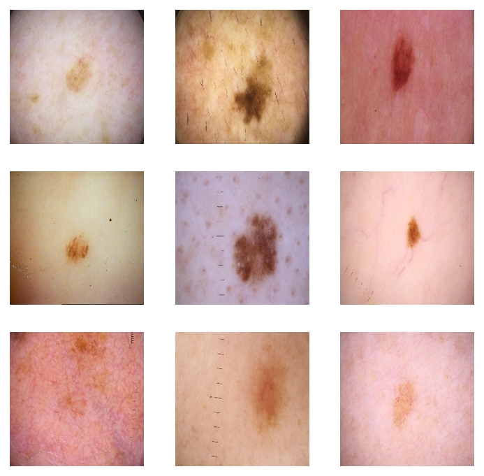
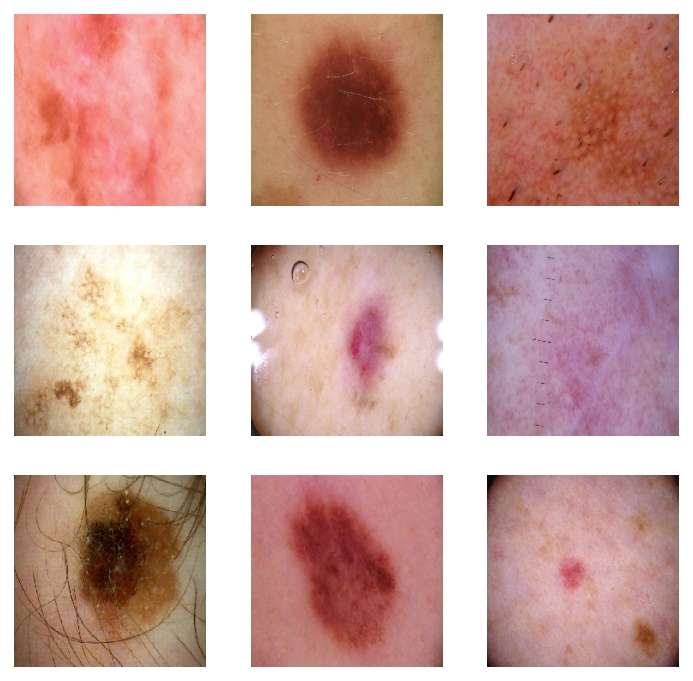
Let’s take a look at the sample images of both classes.

def plot_images(data, target, nrows=3, ncols=3):
    data = data[data['target'] == target].sample(nrows * ncols)['image_path']
    plt.figure(figsize=(nrows * 2, ncols * 2))
    for idx, image_path in enumerate(data):
        image = Image.open(image_path)
        plt.subplot(nrows, ncols, idx + 1)
        plt.imshow(image)
        plt.axis('off')
    plt.show();

# benign samples
plot_images(train_df, target=0)

# malign samples
plot_images(train_df, target=1)

Let’s take a look at the distribution of target class label:

print('% benign: {:.4f}'.format(sum(train_df['target'] == 0) / len(train_df)))
print('% malign: {:.4f}'.format(sum(train_df['target'] == 1) / len(train_df)))

% benign: 0.9824
% malign: 0.0176

Upon analyzing the dataset, it is observed that

• Target class distribution is not balanced, and more samples belong to the benign (majority) class than the malign (minority) class
• If we directly split the dataset into a proportion of say 80:20, then it is possible that the split may not be representative of the actual dataset having the same ratio of the class labels
• This will induce a bias towards predicting the benign class label and thus significantly impact the performance of the classifier

In order to avoid the bias due to an imbalanced dataset and ensure the same distribution of the class labels, we employ the stratified k-fold cross-validation to obtain the same distribution of the class labels in each fold. This cross-validation ensures that we are able to make predictions on all of the data using k different models.

# create folds
n_splits = 5
train_df['kfold'] = -1
train_df = train_df.sample(frac=1).reset_index(drop=True)
train_df_labels = train_df.target.values

skf = StratifiedKFold(n_splits=n_splits)

for fold_idx, (train_idx, valid_idx) in enumerate(skf.split(X=train_df, y=train_df_labels)):
    train_df.loc[valid_idx, 'kfold'] = fold_idx

train_df.to_csv('train_folds.csv', index=False)

Now let’s create a custom data loader to load the data from the specified image paths; it is also capable of performing transformations(if required), directly at the loading stage, so we don’t need to worry about the transformations at later stages.

class MelanomaDataset(torch.utils.data.Dataset):
    def __init__(self, image_paths, targets, resize, augmentations=None):
        """
        Initialize the Melanoma Dataset Class
        """
        self.image_paths = image_paths
        self.targets = targets
        self.resize = resize
        self.augmentations = augmentations
    
    def __getitem__(self, index):
        """
        Returns the data instance from specified index location
        """
        image_path = self.image_paths[index]
        target = self.targets[index]
        
        # open the image using PIL
        image = Image.open(image_path)
        
        if self.resize is not None:
            image = image.resize(
                (self.resize[1], self.resize[0]), resample=Image.BILINEAR
            )
        
        image = np.array(image)

        # perform the augmentations if any
        if self.augmentations is not None:
            augmented = self.augmentations(image=image)
            image = augmented['image']
        
        # make the channel first
        image = np.transpose(image, (2, 0, 1)).astype(np.float32)
        
        return {
            'image': torch.tensor(image),
            'target': torch.tensor(target)
        }

    def __len__(self):
        """
        Returns the number of examples / instances
        """
        return len(self.image_paths)

Evaluation Metrics

The area under the ROC curve (AUC) was used as an evaluation metric for the problem due to an imbalanced dataset. A ROC curve (receiver operating characteristic curve) is a graph showing the performance of a classifier at various classification thresholds. It is a measure of how well the model is capable of distinguishing between the different classes. This curve plots two parameters:

• True Positive Rate (TPR) is a synonym for recall and is therefore defined as follows:

\[{TPR = \frac{TP}{TP + FN}}\]

• False Positive Rate (FPR) is defined as follows:

\[{FPR = \frac{FP}{FP + TN}}\]

AUC is a measure of the area underneath the entire ROC curve. It represents the degree of separability. It ranges in value from 0 to 1. The higher the AUC, the better the model is at distinguishing classes.

For more details, please refer to the Classification: ROC Curve and AUC by Google’s Machine Learning Crash Course.

Losses

We use the Binary Cross Entropy (BCE) loss for the problem since here we need to classify the images into classes: benign or malignant. The formula of the BCE loss is as given below:

\[L = -\frac{1}{N}\sum_{i=1}^N{(y_i\log(p_i) + (1 - y_i)\log(1 - p_i))}\]

where $y_i$ is the class label (0 for benign and 1 for malign) and $p_i$ is the predicted probability of the image being malign for the $i^{th}$ sample

We will use the nn.BCEWithLogitsLoss directly from the PyTorch’s nn module.

Another loss that we try for the problem is the Focal loss, an extension of BCE loss that tries to handle class imbalance by penalizing the misclassified examples. It is expressed as follows:

\[L = -\alpha_t(1 - p_t)^\gamma\log(p_t\] \[\alpha_t= \left\{\begin{matrix} \alpha & if \; y = 1\\ 1 - \alpha & otherwise \end{matrix}\right.\]

where $\gamma$ is a prefixed positive scalar value and $\alpha$ is a prefixed value between 0 and 1 to balance the positive labeled samples and negative labeled samples.

class FocalLoss(nn.Module):
    def __init__(self, alpha=1, gamma=2):
        """
        Initialize the Focal Loss Class
        """
        super(FocalLoss, self).__init__()
        self.alpha = alpha
        self.gamma = gamma
    
    def forward(self, predictions, targets):
        """
        Calculates the Focal Loss
        """
        criterion = nn.BCEWithLogitsLoss()
        
        logits = criterion(predictions, targets.view(-1, 1).type_as(predictions))
        pt = torch.exp(-logits)
        
        focal_loss = self.alpha * (1 - pt) ** self.gamma * logits
        
        return torch.mean(focal_loss)

Network

Convolutional Neural Networks are very good at the task of image processing and classifications due to the following reasons:

• Require fewer parameters i.e. less complex than feed forward networks (FFNs) but are able to achieve as efficient or even better performance
• Able to identify the low-level features such as edges as well as high-level features such as objects or patterns

Here we try the following two different network architectures:

• EfficientNet
• Squeeze and Excitation Network

EfficientNet

The EfficientNet architecture by Tan et al. focuses on scaling up the performance of traditional CNNs in terms of accuracy and at the same time, focuses on building a more computationally efficient architecture.

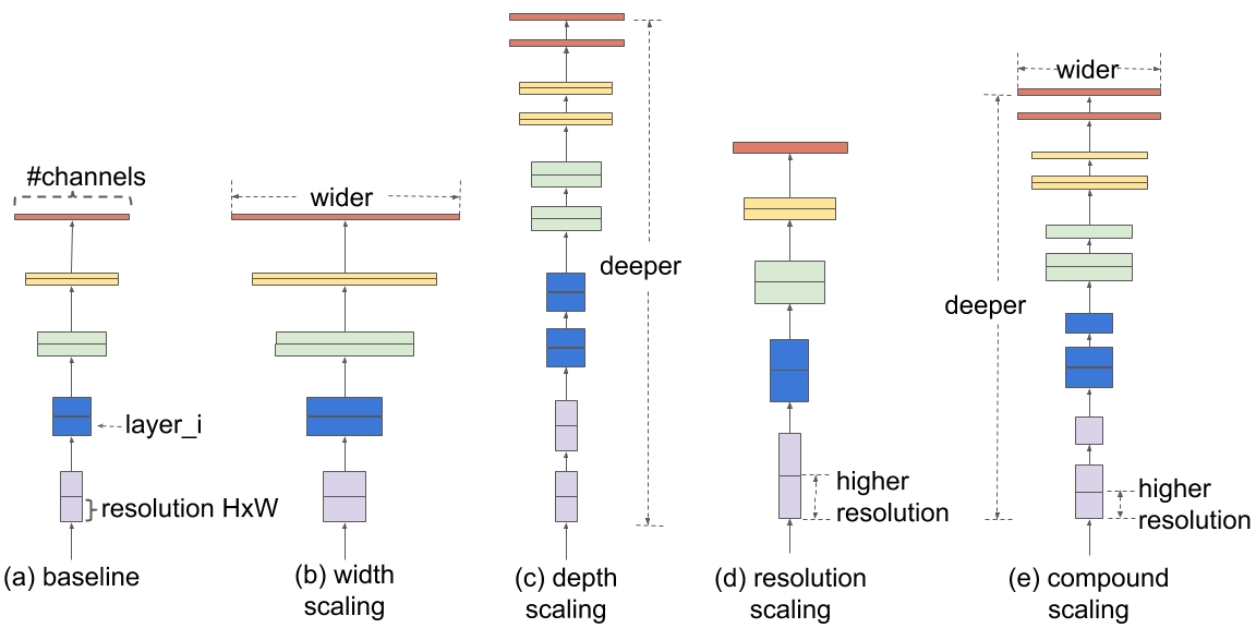
How can CNNs be Scaled up?

Types of Model Scaling (image source)

Here compound scaling is the method proposed by Tan et al.

Let’s first analyze how traditional scaling works and why each type of scaling is necessary.

• Width Scaling (w): The objective of using a wider network is that wider networks are more suited to capture more fine-grained features. This is typically used in shallow networks. But the problem is that if we make the network extremely wide, the performance of the network in terms of accuracy degrades. Therefore, we need an optimum width to maintain performance.

• Depth Scaling (d): Theoretically, deeper neural networks tend to capture more complex features and this makes the neural network generalize well to other tasks. But practically, if we go on making the network too deep, it will increase the computational complexity and such networks will require huge training times. Also very deep neural networks suffer from vanishing/exploding gradient problems. Therefore, we need an optimum depth to achieve good performance.

• Resolution Scaling (r): By intuition, we can consider that if we take a high-resolution image, it would yield more fine-grained features and thus would boost the performance. Though this is true to a certain extent, we cannot assume a linear relationship between these. This is because the accuracy gain diminishes very quickly. So to a certain extent, by resolution scaling, we can improve the performance of the network.

Based on their study, the authors have considered that all these 3 factors should be considered to a certain extent and a combined scaling technique must be incorporated.

By intuition, if we are considering a high-resolution image, naturally, we have to increase the depth and the width of the network. To validate this intuition, the authors considered a fixed-width network (w) and varied the scaling factors r and d. It was observed that the accuracy improved when high-resolution images were passed through deeper neural networks.

The authors have proposed a scaling technique which uses a compound coefficient $\phi$ in order to scale the width, depth and resolution of the network in a uniform fashion, which is expressed as follows:

\[{depth: d = \alpha^\phi}\] \[{width: w = \beta^\phi}\] \[{resolution: r = \gamma^\phi}\] \[such\ that\ \alpha\cdot\beta^2\cdot\gamma^2\approx2\ and\ \alpha,\ \beta,\ \gamma\ \geq 1\]

where $\phi$ is a use r-specified coefficient which can control how many resources are available and $\alpha$, $\beta$, $\gamma$ controls depth, width, image resolution, respectively.

Firstly, for B0, the authors have fixed $\phi = 1$ and have assumed that twice more resources are available and have performed a small grid search for the other parameters. The optimal values which satisfy $\alpha\cdot\beta^2\cdot\gamma^2\approx2$, were found out to be $\alpha = 1.2$, $\beta = 1.1$ and $\gamma = 1.15$.

Later, the authors kept these values of $\alpha$, $\beta$, $\gamma$ as constant and experimented with different values of $\phi$. The authors experiment with different values of $\phi$ to produce the variants EfficientNets B1-B7.

For more details, please refer to the EfficientNet paper.

class Net(nn.Module):
    def __init__(self, variant='efficientnet-b2'):
        """
        Initializes pretrained EfficientNet model
        """
        super(Net, self).__init__()
        self.base_model = EfficientNet.from_pretrained(variant)
        self.fc = nn.Linear(self.base_model._fc.in_features, 1)
    
    def forward(self, image, target):
        """
        Returns the result of forward propagation
        """
        batch_size, _, _, _ = image.shape
        out = self.base_model.extract_features(image)

        out = F.adaptive_avg_pool2d(out, 1).view(batch_size, -1)
        out = self.fc(out)
        
        # loss = nn.BCEWithLogitsLoss()(out, target.view(-1, 1).type_as(out))
        loss = FocalLoss()(out, target.view(-1, 1).type_as(out))
        
        return out, loss
    
model = Net()

Squeeze and Excitation Networks

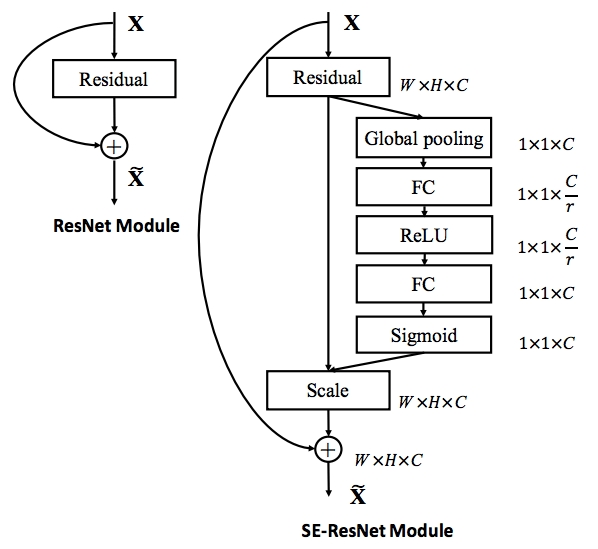
Traditional convolutional neural networks (CNNs) use convolution operation which fuses information both spatially and channel-wise, but Jie Hu et al. proposed a novel architecture Squeeze and Excitation Networks (SENets) in the 2017 ImageNet challenge that focuses on the channel-wise information correlation. This network improved the results from the previous year by 25%.

The basic intuition behind this approach was to adjust the feature map channel-wise by adding the parameters to each channel of a convolutional block. These parameters represent the relevance of each feature map to the information, much like we use attention in the recurrent neural networks (RNNs).

Squeeze and Excitation Block (image source)

The above figure represents the Squeeze-and-Excitation (SE) block where it performs a series of operations: squeeze and excitation, which allows the network to recalibrate the channel-wise information i.e. emphasize informative feature maps and suppresses less useful feature maps. The squeeze operation produces a channel descriptor expressive of the whole image by aggregating feature maps across the spatial dimensions using global average pooling. The excitation operation produces channel-wise relevance using the two fully-connected (FC) layers where the FC captures channel-wise dependencies. This block can be directly applied to the existing architectures such as ResNet, which is shown below.

Residual module (left) and SE ResNet module (right) (image source)

The computational overhead of the network depends on where you apply the SE block. There was a minor increase in the computational overhead, which is feasible compared to the performance boost achieved from the network. The authors applied the SE block at earlier layers to reduce the computation overhead since, at later layers, the number of parameters increases as the feature maps increase channel-wise.

For more details, please refer to the Squeeze-and-Excitation Networks paper.

class Net(nn.Module):
    def __init__(self):
        """
        Initializes pretrained EfficientNet model
        """
        super(Net, self).__init__()
        self.base_model = pretrainedmodels.se_resnext50_32x4d(pretrained='imagenet')
        self.fc = nn.Linear(2048, 1)
    
    def forward(self, image, target):
        """
        Returns the result of forward propagation
        """
        batch_size, _, _, _ = image.shape
        out = self.base_model.features(image)

        out = F.adaptive_avg_pool2d(out, 1).view(batch_size, -1)
        out = self.fc(out)
        
        # loss = nn.BCEWithLogitsLoss()(out, target.view(-1, 1).type_as(out))
        loss = FocalLoss()(out, target.view(-1, 1).type_as(out))
        
        return out, loss
    
model = Net()

Training and Prediction

Here, we use early stopping and learning rate scheduler for training the model faster.

def train(fold):
    """
    Train the model on a fold
    """

    n_epochs = 50
    train_bs = 32
    valid_bs = 16
    best_score = -np.Inf
    es_patience = 5
    patience = 0
    model_path = './model_fold_{:02d}.pth'.format(fold)

    train_folds_df = pd.read_csv(train_folds_df_path)
    train_df = train_folds_df[train_folds_df.kfold != fold].reset_index(drop=True)
    valid_df = train_folds_df[train_folds_df.kfold == fold].reset_index(drop=True)
    
    train_images = train_df.image_path.values
    train_targets = train_df.target.values
    valid_images = valid_df.image_path.values
    valid_targets = valid_df.target.values

    model = Net()
    model.to(device)

    mean = (0.485, 0.456, 0.406)
    std = (0.229, 0.224, 0.225)

    # augmentations for train and validation images
    train_aug = albumentations.Compose([
        albumentations.Normalize(mean, std, max_pixel_value=255.0, always_apply=True),
        albumentations.ShiftScaleRotate(shift_limit=0.0625, scale_limit=0.1, rotate_limit=15),
        albumentations.Flip(p=0.5),
    ])

    valid_aug = albumentations.Compose([
        albumentations.Normalize(mean, std, max_pixel_value=255.0, always_apply=True),
    ])

    # creating dataset and dataloader for train and validation images
    train_dataset = MelanomaDataset(
        image_paths=train_images,
        targets=train_targets,
        resize=None,
        augmentations=train_aug
    )
    train_loader = torch.utils.data.DataLoader(
        train_dataset, batch_size=train_bs, shuffle=True, num_workers=4
    )

    valid_dataset = MelanomaDataset(
        image_paths=valid_images,
        targets=valid_targets,
        resize=None,
        augmentations=valid_aug
    )
    valid_loader = torch.utils.data.DataLoader(
        valid_dataset, batch_size=valid_bs, shuffle=False, num_workers=4
    )

    optimizer = torch.optim.Adam(model.parameters(), lr=3e-4)
    scheduler = torch.optim.lr_scheduler.ReduceLROnPlateau(
        optimizer,
        patience=3,
        threshold=0.001,
        mode='max'
    )

    for epoch in range(n_epochs):
        train_loss = 0
        valid_loss = 0
        train_steps = 0
        valid_steps = 0
        
        # model in train mode
        model.train()

        tk0 = tqdm(train_loader, total=len(train_loader), position=0, leave=True)
        
        with torch.set_grad_enabled(True):
            for idx, data in enumerate(tk0):

                # load tensor to GPU
                for key, value in data.items():
                    data[key] = value.to(device)
                
                # forward pass
                _, loss = model(**data)

                # backward pass, optimize
                optimizer.zero_grad()
                loss.backward()
                optimizer.step()

                train_loss += loss.item()
                train_steps += 1

                # update progress bar
                tk0.set_postfix(loss=train_loss/train_steps)

        tk0.close()

        # model in eval mode
        model.eval()
        val_predictions = np.zeros((len(valid_df), 1), dtype=np.float32)

        tk0 = tqdm(valid_loader, total=len(valid_loader), position=0, leave=True)

        with torch.no_grad():
            for idx, data in enumerate(tk0):

                # load tensor to GPU
                for key, value in data.items():
                    data[key] = value.to(device)
                
                # model prediction
                batch_preds, loss = model(**data)

                start = idx * valid_bs
                end = start + len(data['image'])
                val_predictions[start:end] = batch_preds.cpu()
                
                valid_loss += loss.item()
                valid_steps += 1
                
                # update progress bar
                tk0.set_postfix(loss=valid_loss/valid_steps)
        
        tk0.close()

        # schedule learning rate
        auc = roc_auc_score(valid_df.target.values, val_predictions.ravel())
        print('Epoch = {} , AUC = {}'.format(epoch, auc))
        scheduler.step(auc)

        # early stopping
        if best_score < auc:
            print('Validation score improved ({} -> {}). Saving Model!'.format(best_score, auc))
            best_score = auc
            patience = 0
            torch.save(model.state_dict(), model_path)
        else:
            patience += 1
            print('Early stopping counter: {} out of {}'.format(patience, es_patience))
            if patience == es_patience:
                print('Early stopping! Best AUC: {}'.format(best_score))
                break

def predict(fold):
    """
    Model predictions on a fold
    """

    test_bs = 16
    model_path = './model_fold_{:02d}.pth'.format(fold)
    test_df = pd.read_csv(test_df_path)
    
    test_images = test_df.image_path.values
    test_targets = np.zeros(len(test_images))
    
    model = Net()
    model.load_state_dict(torch.load(model_path))
    model.to(device)
    
    mean = (0.485, 0.456, 0.406)
    std = (0.229, 0.224, 0.225)
    
    # test augmentation on test images
    test_aug = albumentations.Compose([
        albumentations.Normalize(mean, std, max_pixel_value=255.0, always_apply=True),
    ])
    
    # dataset and dataloader for test images
    test_dataset = MelanomaDataset(
        image_paths=test_images,
        targets=test_targets,
        resize=None,
        augmentations=test_aug
    )
    test_loader = torch.utils.data.DataLoader(
        test_dataset, batch_size=test_bs, shuffle=False, num_workers=4
    )
    
    # model in eval mode
    model.eval()
    test_predictions = np.zeros((len(test_df), 1))
    
    tk0 = tqdm(test_loader, total=len(test_loader), position=0, leave=True)

    with torch.no_grad():
        for idx, data in enumerate(tk0):
            
            # load tensor to GPU
            for key, value in data.items():
                data[key] = value.to(device)
                
            batch_preds, _ = model(**data)
            
            start = idx * test_bs
            end = start + len(data['image'])
            test_predictions[start:end] = batch_preds.cpu()
    
    tk0.close()

    return test_predictions.ravel()

Now, let’s train each fold and save the best model.

for i in range(n_splits):
    train(i)

Great, now we are ready with our models so let’s predict the targets on the test images:

final_predictions = np.zeros((len(test_df), 1)).ravel()
for i in range(n_splits):
    final_predictions += predict(i)

final_predictions /= n_splits

sample = pd.read_csv('./sample_submission.csv')
sample.loc[:, 'target'] = final_predictions
sample.to_csv('submission.csv', index=False)

Results

Here, we had trained 2 models, SEResNeXt50_32x4d and the B2 variant of the EfficientNet model. Both models were trained using the loss functions BCE Loss and Focal Loss and the results are compared and tabulated as follows:

Model	BCE Loss	Focal Loss
SEResNeXt50_32x4d	0.8934	0.8762
EfficientNet B2	0.8972	0.8921
SEResNeXt50_32x4d + EfficientNet B2	0.9019	-

In the 3rd case, we average out the predictions of both the models and assess the performance.

Future Resources

Kaggle notebooks are a great place to learn and adapt to best practices of the experts. Here are the few kernels from the competition you can refer:

• SIIM: d3 EDA, Augmentations and ResNeXt
• Analysis of Melanoma Metadata and EffNet Ensemble
• Triple Stratified KFold with TFRecords

</div>